Stochastical Matching Pursuit
Algorithms
for Bayesian Variable Selection
Ray-Bing Chen, Chi-Hsiang
Paper | Code | Algorithm | Examples
Section 1. Paper and
Presentation
Ø Technique Report:
Chen, R.-B.,
Ø Useful References:
n Chipman, H., Hamada, M. and Wu, C. F. J. 1997. A Bayesian variable selection approach for analyzing designed experiments with complex aliasing, Technometrics, 39, 372-381.
n George, E. I. and McCulloch, R. E. 1993. Variable selection via Gibbs sampling, Journal of the American Statistical Association, 88, 881-889.
n George, E. I. and McCulloch, R. E. 1997, Approaches for Bayesian variable selection, Statistica Sinica, 7, 339-374.
n Mallat, S. G. and Zhang, Z. 1993. Matching pursuit with time-frequency dictionaries, IEEE Transactions on Signal Processing, 41, 3397-3415.
n Shao, J. and Chow, S.-C. 2007. Variable screening in predicting clinical outcome with high-dimensional microarrays, Journal of Multivariate Analysis, 98, 1529-1538.
n Smith, M. and Kohn, R. 1996. Nonparametric regression using Bayesian variable selection, Journal of Econometrics, 75, 317-343.
n Wolfe, P. J., Godsill, S. J. and Ng, W. J. 2004. Bayesian variable selection and regularization for time-frequency surface estimation, J. Roy. Statist. Soc. B, 66, 575-589.
The code in this section is more readable and up-to-date than the codes in Section 4. You can start reading from the file "ReadMeFirst".
Basic Version 1: November 20, 2009 (The MATLAB codes for SMP)
Basic Version 2: December 11, 2009 (The MATLAB codes for componentwise Gibbs sampler and SMP)
Section
3.
Stochastic Matching Pursuit Algorithm
Suppose that Y is the variable of interest, and X1, …, Xp are potential independent variables (regressors). The problem of variable selection is to select the “best” subset of X1, …, Xp to model Y. The statistical model is assumed to be a simple linear model,

where Y is an n × 1 response vector,  is an n × p potential model matrix, and Xi is the ith potential variables. Here
 is a
is a  vector of unknown
coefficients and the noise vector
vector of unknown
coefficients and the noise vector follows a multivariate normal distribution with zero
mean vector and covariance matrix,
follows a multivariate normal distribution with zero
mean vector and covariance matrix, .
.
Stochastic Matching Pursuit
Algorithm:
In our Bayesian selection methods, indicate
variables, are used for indicating the ith
variable in the final model or not, and let γ = (γ1, ..., γp)T. Here the prior of
are used for indicating the ith
variable in the final model or not, and let γ = (γ1, ..., γp)T. Here the prior of is independently set to be

For the other priors, we assume that

where pi = P(γi = 0). WLOG, we would set that pi = ρ for all i =1, ..., p. Then in Bayesian variable selection methods, we like to use an MCMC approach to sequentially generate β(j), γ(j) and σ(j), j = 1, 2, 3, ..., from their conditional posterior distributions. Finally the best subset of variables can be determined by the information of {γ(j)}.
In order to save the computing cost, we
would sample  , i = 1, ..., p, instead
of generating β(j), γ(j)
sequentially. Therefore we propose the following a selection algorithm based on
the idea of Matching Pursuit that is proposed by Mallat
and Zhang (1993) and is widely used in signal and image representation. First the
componentwise Gibbs sampler is proposed. However, if the variables are
highly correlated and if the residual variance is small, then an inferior
variable can be visited first and then selected, thus preventing a variable of
more importance from being selected. To solve these possible problems, we
proposed another stochastic matching pursuit by incorporating Metropolis scheme
that consists of a pair of reversible moves: addition and deletion. First the
acceptance probability for the proposal of adding variable i whose current γi = 0
is
, i = 1, ..., p, instead
of generating β(j), γ(j)
sequentially. Therefore we propose the following a selection algorithm based on
the idea of Matching Pursuit that is proposed by Mallat
and Zhang (1993) and is widely used in signal and image representation. First the
componentwise Gibbs sampler is proposed. However, if the variables are
highly correlated and if the residual variance is small, then an inferior
variable can be visited first and then selected, thus preventing a variable of
more importance from being selected. To solve these possible problems, we
proposed another stochastic matching pursuit by incorporating Metropolis scheme
that consists of a pair of reversible moves: addition and deletion. First the
acceptance probability for the proposal of adding variable i whose current γi = 0
is
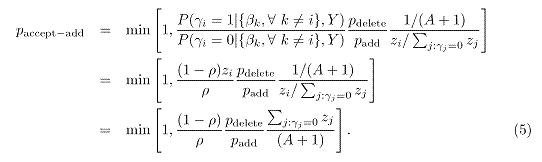
The acceptance probability for the proposal of deleting variable i whose current γi = 1 is
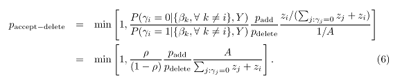
Thus the Algorithm 2 is our stochastic matching pursuit algorithm for variable selection.
Bayesian Variable Selection
Procedure:
Based on the idea of matching pursuit algorithm, we wan to propose a stochastic algorithm such that we can generate {γ(j)} that converges weakly to the posterior distribution, π(γ|Y). After discarding the first M samples, the remaining sequence of γ can be used to compute the posterior probability, π(γ|Y). Then based on the median probability criterion, the “best” model can be determined by the information of γ(j), j > M. The details of our procedure is in the following:
1. Choose the proper parameters, ρ and τ, for stochastic matching pursuit.
2. Stochastic matching pursuit is used for generating posterior sequence of {γ(j)}.
3. Select the best model according to the median probability criterion.
Tuning Parameter Selection:
WLOG, we assume ρ= pi = P(γi = 0), and τ = τi for all i = 1, …, p.
1 For choosing ρ: Usually we would set ρ= 0.5, because we have no information about which variable should be in the model or not.
2 For the parameter τ: The larger τ is, the small the conditional probability of γi = 1 is. To select a proper τ, our suggestion is that 10 < τ < 100. Otherwise the CV type methods can be used for selection, and we would suggest K-fold CV or MCCV to select τ by minimizing the 2-norm prediction errors.
Section 4: Reproducing Examples
Large
n and Small p problems:
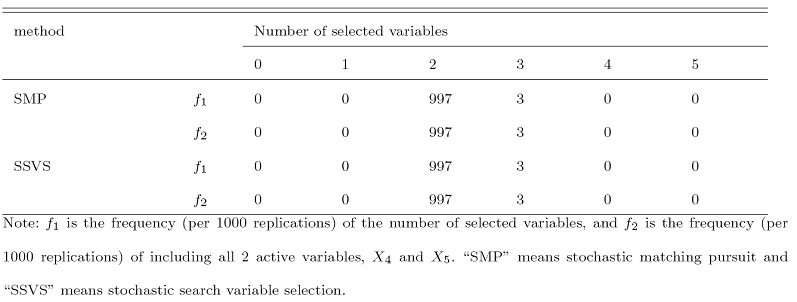
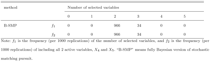
Here we consider the cases that n > p, i.e. there are more observations than the number of candidate regressors. Three simulations and one real example are studied here. The first simulation is the same as what George and McCulloch (1993) did. In the inverse gamma prior of σ2, we set ν = 0 and λ = 1. In the following tables, f1 means the number of remaining variables after selecting, and f2 is the number of remaining regressors that include the true model.
Example 1
In this example, (n, p) = (60, 5). We generate  and let
  . Then response vector, Y = [X1,...,
X5]β + ε, where ε ~MN(0, I60).
To apply SMP, we set (ρ, τ) = (0.5, 15). We also code SSVS by
ourselves and in our SSVS, we set the parameters, (ν0, c), to
be (0.01, 2500). After 1000 replications, the results are summarized in the
following table.
. Then response vector, Y = [X1,...,
X5]β + ε, where ε ~MN(0, I60).
To apply SMP, we set (ρ, τ) = (0.5, 15). We also code SSVS by
ourselves and in our SSVS, we set the parameters, (ν0, c), to
be (0.01, 2500). After 1000 replications, the results are summarized in the
following table.
The corresponding MATLAB code and data
l
The selection results that τ is chosen by the 5-fold CV approach:
The value of τ can also be selected via CV approach. Give the candidate set of τ to be {10, 20, …, 50}. The 5-fold CV approach is used to select the proper value of τ first and then SMP is applied to identify the final model. Based on the same data set, the selection results with 1000 replications are as follows.
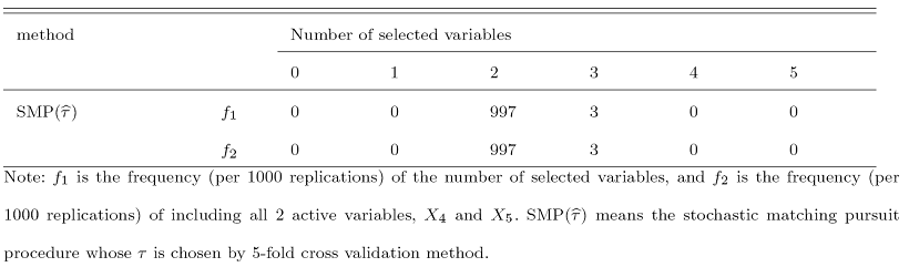
From this table, the selection results are the same as what we do with a fixed τ = 15.
Example 2
In this example, (n, p) = (60, 10). We generate  and the response
vector
and the response
vector
Y = 2 X1 + 3 X2 + 4 X5 + 5 X6 + 6 X9 + 7 X10 + ε.
To apply SMP, we set (ρ, τ) = (0.5, 15). In our SSVS, we set the parameters, (ν0, c), to be (0.01, 2500). After 1000 replications, the results are summarized in the following table.
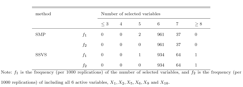
The corresponding MATLAB code and data
l
The selection results that τ is chosen by the 5-fold CV approach:
The value of τ can also be selected via CV approach. Give the candidate set of τ to be {10, 20, …, 50}. The 5-fold CV approach is used to select the proper value of τ first and then SMP is applied to identify the final model. Based on the same data set, the selection results with 1000 replications are as follows.
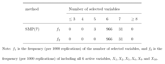
Small
n and Large p problems:
Example 3: A simulation study
Here we consider the situation that we only have fewer observations than the number of candidate regressors, i.e. n < p. In this simulation study, the candidate regressor is
Xi = Gi + k G,
where Gi, i = 1,
..., p and G are iid from multivariate normal distribution
with zero mean vector and covariance matrix, In, and k
is a pre-specified variable. To obtain the response vector, Y, the coefficient
vector β is defined to be  and the corresponding error term is assumed to be ε ~MN(0, In).
Thus there are only five active regressors.
and the corresponding error term is assumed to be ε ~MN(0, In).
Thus there are only five active regressors.
In SMP, besides we fix ρ =
0.5, we select  by 5-fold CV from {80, 120, 160, 220} for k = 0
and {100, 150, 200, 250} for k = 1. We compare our results
with a variable screening method proposed by Shao and
Chow (2007), which is similar to the idea of LASSO. The results are shown in
the following two tables. In tables, “SC” means the method of Shao and Chow (2007). f1
is the number of remaining regressors after
selecting, and f2 is the number of remaining regressors that are related to the response. If the number
of remaining regressors is less than 5, then f2
is the number of remaining variables are in {X1, ..., X5}. Finally we also compare our
selection results with a Lasso type method, which is available from http://www.stat.berkeley.edu/twiki/Research/YuGroup/Software.
In this tool box, the function lasso_cv can be used
for estimating the unknown parameters in the linear models. Thus the selection
variables for this function, lasso_cv, are included
into the model if the corresponding coefficient estimations are no-zeros.
by 5-fold CV from {80, 120, 160, 220} for k = 0
and {100, 150, 200, 250} for k = 1. We compare our results
with a variable screening method proposed by Shao and
Chow (2007), which is similar to the idea of LASSO. The results are shown in
the following two tables. In tables, “SC” means the method of Shao and Chow (2007). f1
is the number of remaining regressors after
selecting, and f2 is the number of remaining regressors that are related to the response. If the number
of remaining regressors is less than 5, then f2
is the number of remaining variables are in {X1, ..., X5}. Finally we also compare our
selection results with a Lasso type method, which is available from http://www.stat.berkeley.edu/twiki/Research/YuGroup/Software.
In this tool box, the function lasso_cv can be used
for estimating the unknown parameters in the linear models. Thus the selection
variables for this function, lasso_cv, are included
into the model if the corresponding coefficient estimations are no-zeros.
l
The results based on 100 replications for (n, p) = (50, 200)
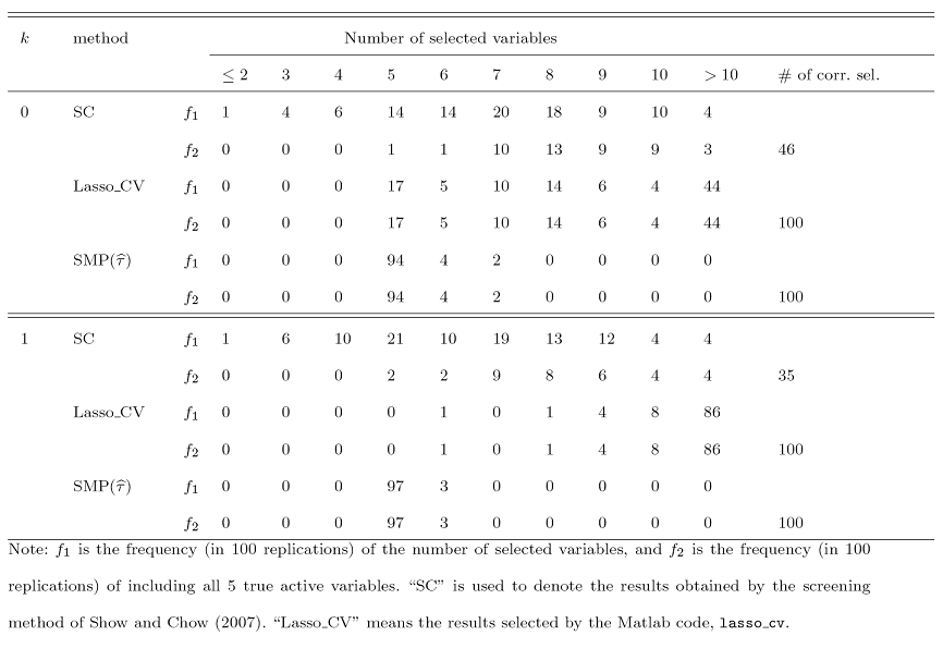
l
The results based on 100 replications for (n, p) = (100, 400)
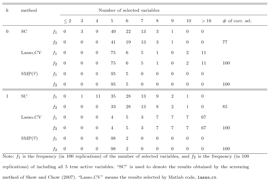
The
corresponding MATLAB code and data
Example 4: Image
representation
Now we apply our selection procedure into the image representation
problem via Gabor regression (Wolf et al., 2004). Totally there are 100 grid
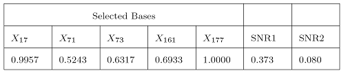
points and there are 200 Gabor bases in our candidate set. X17, X71,
X161 and X177 are active regressors
by setting β17 = 7, β71 = -7, β161
= 7, β177 = -7 and βi
= 0 for the other regressors. Here we select  by MCCV with 100
replications from A = {50, 100, ...,
300}. The selected regressor with the corresponding posterior probabilities are show in
the following table. Here
by MCCV with 100
replications from A = {50, 100, ...,
300}. The selected regressor with the corresponding posterior probabilities are show in
the following table. Here

where  is the predicted values, and Ytrue
is the response vector without noise.
is the predicted values, and Ytrue
is the response vector without noise.
l
The
posterior inclusion probability of the selected bases
The Fully Bayesian Version:
Before running our code, we still need to specify some prior parameters for the prior distribution, for example, τ in the prior of βi. Another possible approach is to set priors for these parameters and then sample them in the MCMC process. Here an inverse gamma prior with parameters, κ and ξ, is chosen for τ. Then we modify Step (VI) in Algorithm 2 by adding a step for τ to sample from its posterior inverse gamma distribution. Two simulations are used to show the performances of this full Bayesian version.
l Large n and Small p problem in Example 1: Here we set (κ, ξ) = (1, 10).
l
Small n and Large p problem in Example 3 with (n, p) =
(50, 200): We also fix (κ, ξ) = (1, 10).
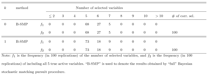
From these two results show that our fully Bayesian version of stochastic matching pursuit algorithm works for both cases. However, we still need to pre-specify the prior parameters, κ and ξ, for the prior of τ.