Overcomplete Blind Source Separation For Time-series Processes
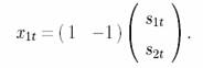
We consider the overcomplete situation, i.e. more sources than the receivers, and there is no noise in the observations. Hence the model is
![]()
where xt=(x1t,…,xmt)¢ is a receiver
vector at time t, st=(s1t,…,sMt)¢ is a source
vector at time t, and A is an m´M matrix
with M > m.
Here we develop a MCMC algorithm to recover the sources and to estimate
the unknown mixing matrix only from the observations. Let Singular Value
Decomposition (SVD) of A is A = U(D 0)V¢ = U(D 0)(V1
V2) ¢. Then the source can be solved
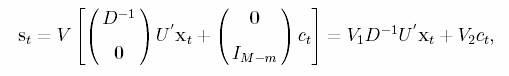
where V1
is the basis for the row space of A, and V2 is a basis for the null
space of A. Assume the joint density of sources is P(s1,…,sT).
Then the joint density of x1…xT and c1…cT
is
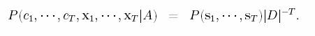
Now this problem
can be treated in a Bayesian framework by putting the uniform priors on U and
V, and uniform priors on log(D). Hence x1,…,xT
are observation data, c1,…,cT are missing
data, and A=U(D 0)V¢ is the unknown
parameter.
The computation
can be accomplished by the data augmentation algorithm of Tanner and Wong
(1987).
- Recovering st by sampling
from P(c1,…,cT|x1,…,xT,A)
(Inhibition Algorithm)
Let P(c1,…,cT|x1,…,xT,
A) µ exp(-H(c)). Then sampling is accomplished by
Langenvin-Euler movers: at the (t+1)th iteration,

where Zt is the white noise, and h is the step
size.
2.
Estimating
A by sampling from P(U,V,log(D)|x1,…,xT,c1…,cT)
(Givens Sampler)
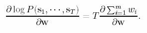
a.
log D:
Let wi = log di and w = (w1,…,wm)¢. Then w1,…,wm
are solved by the following equation:
b.
The
orthogonal matrices, U and V: We repeated Givens rotation for any two columns
of U and V. For example, we want to update U, and randomly pick two columns, ui
and uj. Then
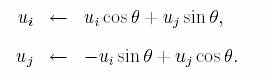
The angle q
is sampled from
![]()
Example 1
Here the sound signals are modeled as the Autoregressive process with order d, i.e.
![]()
where ![]() are autoregressive coefficients and zit
are i.i.d. normal distribution with mean 0 and variance s2i.
are autoregressive coefficients and zit
are i.i.d. normal distribution with mean 0 and variance s2i.
Assume all sources are AR(8) models, and all AR coefficients are
known. The observations are mixed by
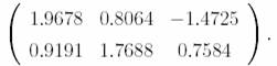
After 100 iterations, the estimated matrix is
![]()
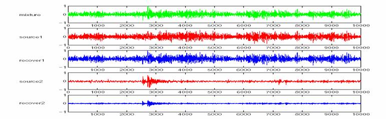
Sound files: Mixture
Source 1 Source 2 Recover 1 Recover 2
Example 2:
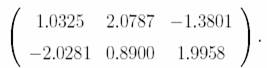
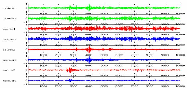
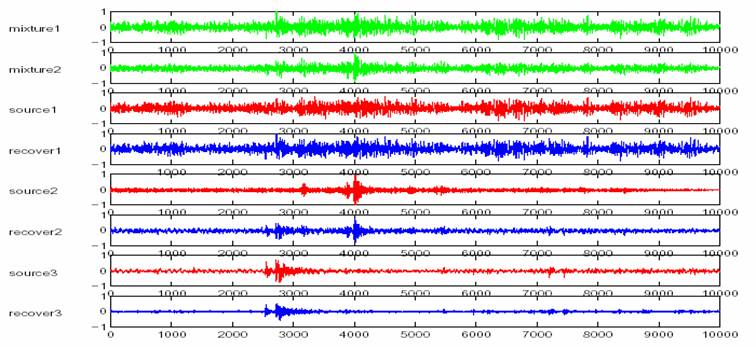
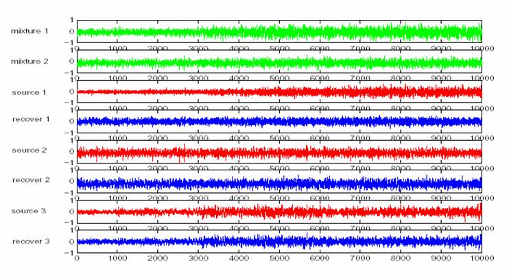
We assume that we have three original sources, and all sources are AR(8) models with known AR coefficients. The observations are mixed by

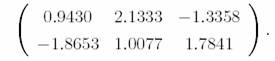
After 200 iterations, the estimated matrix is
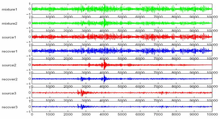
Sound files: Mixture 1 Mixture 2 Source 1 Source 2 Source 3 Recover 1 Recover 2 Recover 3
Example 3:
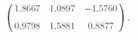
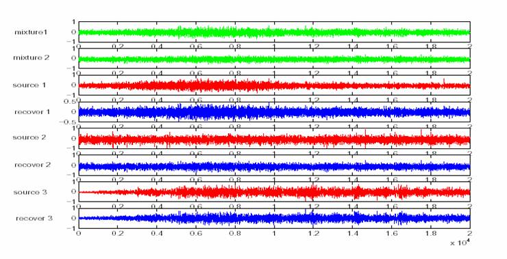
We assume that we have three original sources, and all sources are AR(8) models with known AR coefficients. The observations are mixed by

After 200 iterations, the estimated matrix is
Sound files: Mixture 1
Mixture 2 Source 1 Source 2 Source 3 Recover 1 Recover 2 Recover 3
Example 4:
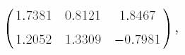
We assume that we have three original sources, and all sources are AR(8) models with known AR coefficients. The observations are mixed by
After 160 iterations, the
estimated matrix is
Sound files: Mixture 1 Mixture 2 Source 1 Source 2 Source 3 Recover 1 Recover 2 Recover 3
Example 5:
We
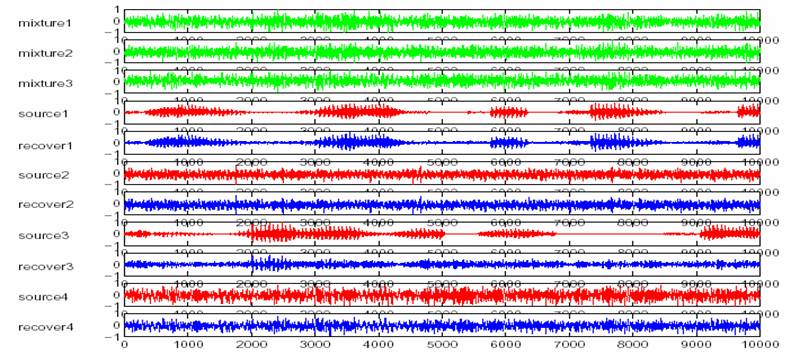
assume that we have four original sources, and all sources are AR(8) models with
known AR coefficients. The observations
are mixed by

After
250 iterations, the estimated matrix is
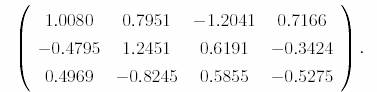
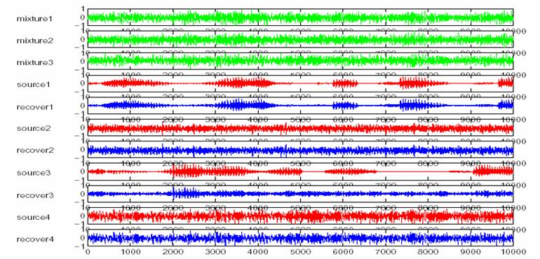
Sound files: Mixture 1 Mixture 2 Mixture 3 Source 1 Source 2 Source 3 Source 4 Recover 1 Recover 2 Recover 3 Recover 4
Example 6:
Here the sound signals are modeled as the Autoregressive and moving average process with order (p,q), i.e.
![]()
where ![]() are autoregressive coefficients ;
are autoregressive coefficients ; ![]() are moving average coefficients and zit are i.i.d. normal
distribution with mean 0 and variance s2i.
are moving average coefficients and zit are i.i.d. normal
distribution with mean 0 and variance s2i.
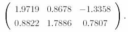
Assume all sources are ARMA(4,2) models, and
all ARMA coefficients are known. The observations are mixed by
After 100 iterations, the estimated matrix is
![]()
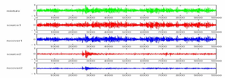
Sound files: Mixture Source 1 Source 2 Recover 1 Recover 2
Example 7:
We
assume that we have three original sources, and all sources are ARMA(4,2) models with known ARMA coefficients. The observations are mixed by
After 200 iterations, the
estimated matrix is
Sound files: Mixture 1 Mixture 2 Source 1 Source 2 Source 3 Recover 1 Recover 2 Recover 3
Example 8:
We
assume that we have three original sources, and all sources are ARMA(4,2)
models with known ARMA coefficients. The observations are mixed by
After 200 iterations, the estimated matrix is

Sound files: Mixture 1 Mixture 2 Source 1 Source 2 Source 3 Recover 1 Recover 2 Recover 3
Example 9:
We
assume that we have four original sources, and all sources are ARMA(5,3) models with known ARMA coefficients. The observations are mixed by
After
250 iterations, the estimated matrix is

Sound files: Mixture 1 Mixture 2 Mixture 3 Source 1 Source 2 Source 3 Source 4 Recover 1 Recover 2 Recover 3 Recover 4
Example 10:
We assume that we have three original sources, and all sources are AR(8) with unknown AR coefficients. The coefficients are estimated in the each iteration by the covariance method. After 340 iterations, the estimated matrix is
and the coefficients are
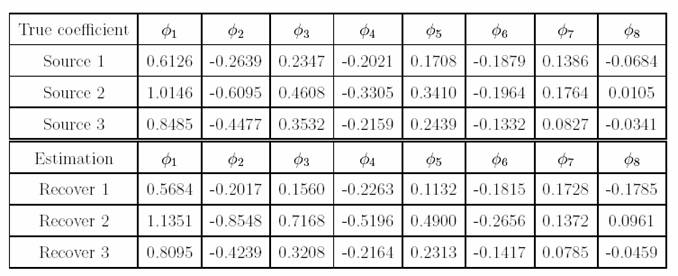
Sound files: Mixture 1 Mixture 2 Source 1 Source 2 Source 3 Recover 1 Recover 2 Recover 3